Session 2· ·keynesian cross
The Keynesian Cross
Short-run demand, consumption functions, and how output adjusts when prices are rigid.
- #keynesian-cross
- #consumption-function
- #multiplier
- #paradox-of-thrift
- #short-run
Session 2 · The Keynesian Cross
LockedSign in with your ISB email to watch this recording.
The clock changes in this session. Session 1 was decades — growth, ponds, patience. Now the horizon shrinks to quarters, prices stop moving, and demand runs the show. This is the machinery behind every stimulus debate you have ever watched — the multiplier, the 45-degree line, the paradox of thrift — built from one equation and pushed until it squeaks, including on GST cuts, tariffs, and Sri Lanka.
Opening & Research Context
Professor Prasanna Tantri opens with research on street vendor financing in emerging markets, presenting data from 1000 treatment and 1000 control groups. This empirical work motivates the shift from long-run growth theory to short-term demand analysis. He references Joel Mokyr’s seminal idea: “ideas create the world.” This philosophical foundation underpins the session’s focus on how expectations and shocks drive output in the short run.
Critical Foundation: Long-Term vs Short-Term
Always distinguish between claims about growth and actual growth drivers.
When someone claims GDP will grow, Professor Tantri emphasizes that we must ask: Will it increase labor supply? Will investment rise? Will technology improve? If none of these fundamentals change, then there is no real growth - only nominal or demand-driven changes.
This distinction is crucial because in the short run (which this session addresses), increases in aggregate demand can raise output even without changes to productive capacity. In the long run, only supply-side improvements matter.
Aggregate Demand vs GDP
Core Distinction
GDP (Y) = What is produced or supplied in the economy
Aggregate Demand (Z) = What people actually want to buy
These two need NOT be equal in the short term. If demand exceeds supply, inventories fall and producers increase output. If supply exceeds demand, inventories build and producers cut output. This dynamic is at the heart of short-run macroeconomics.
Aggregate Demand Decomposition
Z = C + I + G
C(Consumption): Spending on goods and services whose utility is exhausted within one time period.
I(Investment): Spending on capital goods (primarily machinery, equipment, and infrastructure) that provide benefits over multiple periods.
G(Government Spending): Government purchases of goods, services, and public investment.
International Consumption Patterns
| Country | Consumption % of GDP |
|---|---|
| United States | ~70% |
| India | 56-60% |
| China | ~40% |
India’s consumption share has actually GROWN over recent decades. What has fallen is investment as a percentage of GDP, contributing to slower growth despite higher consumption.
Modelling Consumption
The Consumption Function
C = C0 + C1(Y - T)
C0: Autonomous Consumption
Consumption that occurs regardless of current income. Driven by:
-
Borrowing against future income
-
Wealth effects (e.g., when gold prices rise)
-
Expectations about future income
C1: Marginal Propensity to Consume (MPC)
The fraction of each additional rupee of disposable income that is spent on consumption. Constraint: 0 < C1 < 1 (people consume some but not all additional income)
(Y - T): Disposable Income
Income after taxes. Y = national income, T = total taxes.
Key Assumption: Price Rigidity
The Keynesian framework assumes prices are rigid in the extreme short run. This is a foundational assumption that makes demand changes translate into output changes rather than pure price movements. As we move further out, prices become more flexible and the classical model’s predictions dominate.
5. GST Cuts & Stimulus: Real-World Application
Professor Tantri uses GST cuts as a concrete case study to illustrate the model’s implications and limitations.
5.1 The Naive View
Media reports often claim that GST cuts stimulate the economy by increasing consumption. The assumption implicit in this view: reduce T → increase (Y - T) → increase C → increase Z → increase Y.
5.2 The Critical Flaw
When taxes (T) decrease, government revenue also decreases.
Unless the government either:
• Reduces expenditure (G) correspondingly, OR
• Increases borrowing
The stimulus will be incomplete or unsustainable.
5.3 Two Scenarios
Scenario A: G Stays Constant (Deficit Increases)
If government maintains spending while cutting tax revenue:
• Larger fiscal deficit → RBI must finance it or allow inflation → Crowding out of private investment
• If inflation expectations rise, consumption is discouraged → stimulus collapses
Scenario B: G Decreases (Balanced Budget)
If government cuts spending proportionally to maintain budget balance:
• Net effect is ambiguous because both C and G change
• The multiplier effect depends on the relative sizes of these changes
5.4 Real-World Example: Sri Lanka
Sri Lanka provides a cautionary tale. The government cut taxes without corresponding expenditure reductions. The result: larger deficits, inflation expectations rose, and the stimulus collapsed into a severe debt crisis. This demonstrates why the assumption that “any assumption breaks → inflation expectations rise → stimulus collapses” is not merely theoretical but empirically relevant.
Tariff Analysis
Professor Tantri offers a brief but insightful digression on tariffs and pricing:
6.1 The Key Insight
In oligopolistic markets (few large suppliers), firms have pricing power and may absorb tariffs rather than pass them fully to consumers. In competitive markets, tariffs are passed through 1:1 to prices.
6.2 Business Intelligence Application
When tariffs are imposed and prices DON’T rise proportionally, this reveals important information: the market is NOT competitive. High-margin oligopolists are absorbing the cost. This can be valuable intelligence for business strategy and competitive analysis.
7. The Keynesian Cross Equation
This section derives the fundamental equation of the Keynesian model.
7.1 Starting Point
Z = C0 + C1(Y - T) + I-bar + G-bar
7.2 Equilibrium Condition
In equilibrium, aggregate demand equals output:
Y = Z
7.3 Solving for Equilibrium Output
Substituting the consumption function into the demand equation and setting Y = Z:
Y = C0 + C1(Y - T) + I-bar + G-bar
Expanding:
Y = C0 + C1*Y - C1*T + I-bar + G-bar
Collecting Y terms on the left:
Y - C1*Y = C0 - C1*T + I-bar + G-bar
Factoring:
Y(1 - C1) = C0 - C1*T + I-bar + G-bar
7.4 Equilibrium Output (Keynesian Cross Solution)
Y* = (C0 - C1*T + I-bar + G-bar) / (1 - C1)
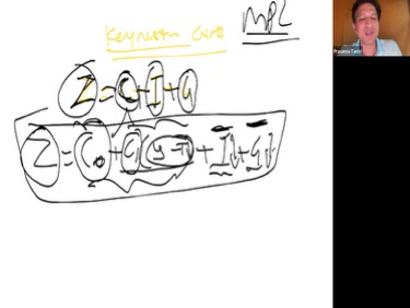
Figure 2: Whiteboard showing the complete consumption function with MPC notation
7.5 The Fiscal Multiplier
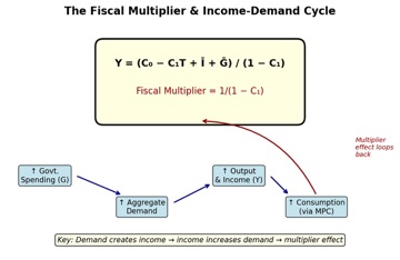
The term 1/(1 - C1) is the Keynesian multiplier. It shows how much output expands for each unit increase in autonomous spending (whether from C0, I-bar, or G-bar).
Example Calculation
If C1 = 0.8:
1. Multiplier = 1 / (1 - 0.8) = 1 / 0.2 = 5
This means: when government increases spending by 1 rupee:
2. Round 1: Spend 1 rupee → income rises by 1
3. Round 2: Consume 0.80 of new income → income rises by 0.80
4. Round 3: Consume 0.80 x 0.80 = 0.64 → income rises by 0.64
5. Round 4: 0.512 → …
Total Output Increase = 1 + 0.80 + 0.64 + 0.512 + … = 5 rupees
Multiplier Interpretation
The multiplier reflects a dynamic process: initial government spending creates income, recipients spend a fraction (the MPC), creating additional income, which is partially spent again, and so on. The cumulative effect amplifies the initial stimulus.
Comparative Statics
Comparative statics examines how equilibrium output changes when parameters shift. Each change is amplified by the multiplier.
Tax Decrease (T Decreases)
Lower taxes → higher disposable income → higher consumption → higher output
Output multiplier: ΔY = C1 x Multiplier x (-ΔT)
Investment Increase (I-bar Increases)
Higher investment → directly increases aggregate demand → output rises by multiplier
Output multiplier: ΔY = Multiplier x ΔI-bar
Government Spending Increase (G-bar Increases)
Higher government spending → directly increases aggregate demand → output rises by multiplier
Output multiplier: ΔY = Multiplier x ΔG-bar
Autonomous Consumption Shift (C0 Increases)
Wealth shock (e.g., gold prices spike) → autonomous consumption rises → output expands by multiplier
Output multiplier: ΔY = Multiplier x ΔC0
In the Keynesian framework, any change in autonomous spending (whether fiscal, investment-driven, or confidence-driven) is amplified through the multiplier mechanism. The MPC is the critical parameter determining multiplier magnitude.
The Keynesian Cross Diagram
Diagram Structure
• X-axis: Income (Y)
• Y-axis: Demand (Z)
Key Lines
• The 45-degree line represents Y = Z (equilibrium locus)
• The aggregate demand curve Z = C0 + C1(Y - T) + I-bar + G-bar has slope C1 (0 < slope < 1), so it is flatter than the 45-degree line
The Equilibrium
The intersection of the aggregate demand curve and the 45-degree line determines equilibrium output Y*. At this point, aggregate demand equals output, so there is no pressure for change.
Below Equilibrium
• When Y < Y*: Z > Y (demand exceeds supply)
• Inventories fall → producers increase output → income rises
• The economy moves rightward along the demand curve toward equilibrium
Above Equilibrium
• When Y > Y*: Z < Y (supply exceeds demand)
• Inventories accumulate → producers decrease output → income falls
• The economy moves leftward along the demand curve toward equilibrium
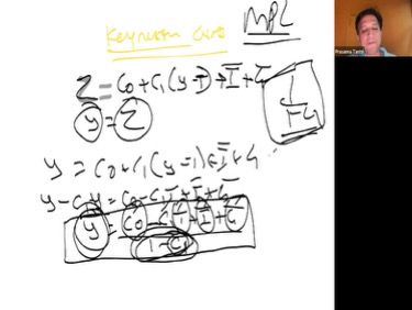
complete equilibrium derivation and the Keynesian Cross diagram
Shifts in Aggregate Demand
Changes in autonomous components (C0, I-bar, G-bar, or taxes) shift the demand curve. The new intersection with the 45-degree line defines the new equilibrium. The change in output is determined by the multiplier and the size of the shift.
Animal Spirits
Animal Spirits: A sudden change in confidence or optimism about the future with no change in fundamentals.
When animal spirits are bullish, C0 rises (consumers borrow and spend more). This shifts the demand curve up, triggering a multiplier-amplified boom. Conversely, pessimistic animal spirits cause a sharp contraction. This mechanism explains why business confidence and consumer sentiment are crucial to macroeconomic fluctuations, independent of changes to productive capacity.
Crucial Assumption: Supply Flexibility
Critical Caveat: The Keynesian model assumes that when demand increases, producers can increase supply without running into constraints. This is valid when there is unemployment and excess capacity.
If the economy is near full capacity, an increase in demand will simply raise prices rather than output. The model’s prediction - that demand drives output - breaks down when supply is constrained.
The Paradox of Thrift
10.1 The Paradox
In the Keynesian framework, increased savings can be BAD for short-run output.
10.2 Mechanism
If households increase their savings rate, they reduce their consumption (lower C1 or increase (1 - C1)). If interest rates do not fall (e.g., the central bank holds rates constant), this reduced consumption:
• Decreases aggregate demand
• Triggers a downward multiplier effect
• Income falls, which can reduce actual savings despite the desire to save more
10.3 The Classical Resolution
The paradox is resolved in the long run if lower savings leads to lower interest rates, which stimulates investment. When investment rises enough to offset consumption’s decline, output returns to trend. However, during the transition (which is what Keynesian analysis focuses on), higher savings can be contractionary.
11. Credit & Delinquency Discussion
Timeline: [46:40 - 50:50]
A student raises a question about unsecured lending: consumers borrowing to purchase items like iPhones or concert tickets. Professor Tantri provides important context.
11.1 Short-Run Effect
When unsecured lending expands, C0 (autonomous consumption) increases because more people can borrow. This directly boosts aggregate demand and output through the multiplier. The short-run stimulus is real.
11.2 Delinquency Risk
However, if delinquencies rise on unsecured loans (borrowers unable to repay), lenders reduce credit supply. This contracts future consumption and aggregate demand.
11.3 Systemic Risk Assessment
Professor Tantri notes that unsecured lending in India currently (~4-5 lakh crores) represents only about 5% of the ~180 lakh crore banking system. Compared to the scale of the 2008 US subprime crisis, this is
• Not yet a systemic threat
• But a risk to monitor
• Potentially important for monetary policy if growth slows
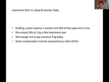
Figure 4: Slide from Session 1 on Investment foundations (for structural context)
Key Takeaways
1. Aggregate Demand Framework
6. Aggregate demand (Z = C + I + G) determines short-run output when prices are rigid. GDP and demand need not be equal; the gap drives inventory and production adjustments.
2. Consumption Function
7. C = C0 + C1(Y - T) separates autonomous consumption from income-dependent consumption. The MPC (C1) is the critical parameter determining multiplier size.
3. Fiscal Multiplier
8. The multiplier = 1/(1 - C1) amplifies shocks. Higher MPC means larger multiplier. Changes in government spending, taxes, or investment are magnified through multiple rounds of spending and income.
4. GST Cuts & Policy Design
9. Tax cuts only stimulate if government spending is maintained and inflation expectations remain anchored. If either assumption breaks, stimulus fails. Sri Lanka’s experience shows real costs of unsustainable fiscal policy.
5. Keynesian Cross Dynamics
10. The intersection of aggregate demand and the 45-degree line (Y = Z) determines equilibrium. Below equilibrium, rising demand boosts output. Above, falling demand contracts output. The economy naturally converges to equilibrium through inventory mechanisms.
6. Paradox of Thrift
11. In the short run, increased savings can reduce consumption → reduce aggregate demand → reduce output. This is only resolved if lower savings rates lead to lower interest rates that stimulate investment.
7. Animal Spirits
12. Sudden shifts in confidence (unrelated to fundamentals) change autonomous consumption and trigger multiplier booms or busts. Business and consumer sentiment are real drivers of macroeconomic fluctuations.
8. Supply-Side Constraint
13. The model assumes slack in the economy (unemployment, excess capacity). If the economy is near full capacity, demand increases drive prices, not output. Policy effectiveness depends critically on the economic slack available.
Session References
Joel Mokyr’s concept that ideas create the world provides the philosophical underpinning. In the Keynesian framework, ideas (expectations, animal spirits) have real economic consequences.
Sri Lanka’s fiscal crisis demonstrates the real costs of violating model assumptions. Tax cuts without expenditure cuts, unsustained by RBI accommodation, led to inflation and debt crisis.
The observation that tariff incidence (whether prices rise proportionally) reveals market structure is a valuable tool for business analysis of competitive dynamics.
Supplementary Notes (From Student’s Handwritten Notes)
Keynesian Way of Consumption
Why would a nation not produce a complete economic approach on a country/world level? Because individuals would only spend that amount which occurs — I surely would not spend money on go or whatever in or abilities.
Savings as a means to grow the economy is why lower interest rates and giving rise — savings could involve long-time horizons.
The Keynesian view: demand drives supply, not the other way around. In the short term, prices are rigid, so when people don’t consume, firms can’t slash prices and clear inventory. Inventory stays put for next quarter and production in subsequent quarters decreases.
The Goods Market Equilibrium
We call 1/(1−C₁) the fiscal multiplier
Aggregate Demand (Z) and Aggregate Output, which we also call GDP (Y)
Z = C + Ī + Ḡ → Z = C₀ + C₁(Y−T) + Ī + Ḡ
Autonomous consumption (C₀) is the baseline consumption regardless of income
MPC (C₁): The marginal propensity to consume
Key assumption: If T (taxes) reduces, even then the government maintains its deficit
The government treats deficit with pure demand for money — raising interest rates
Now RBI will step in to maintain interest rates. They will do VRRs (Variable Rate Repos), i.e., increase money supply
Real Interest Rate = Nominal Rate − Inflation
Endogenous variables move along the graph; exogenous factors shift from outside
The multiplier cycle: Output → Increasing income → Demand creates income → Income increases demand
Equilibrium: Y = (C₀ − C₁T + Ī + Ḡ) / (1 − C₁)
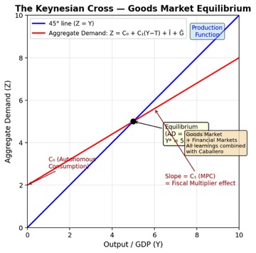
Keynesian Cross — Goods Market Equilibrium (Recreated from handwritten notes)
The Fiscal Multiplier & Debate Around Tax Cuts
The debate around tax cuts leading to increased GDP: The government’s argument is based on the spending argument that MPC of an ordinary citizen is much more than that of a government employee
What happens if people save instead of consuming? Inventory piles up. In the short-term there’s also price rigidity (explore this more)
Key driver of the Keynesian Cross: demand, and supply is thought to be a constant because of price rigidity
The Keynesian view is good in the short-term because assumptions (price rigidity, etc.) are fairly accurate within that time-frame
Production/labour efficiency/human capital constraints apply in the longer run
Fiscal Multiplier & Income-Demand Cycle 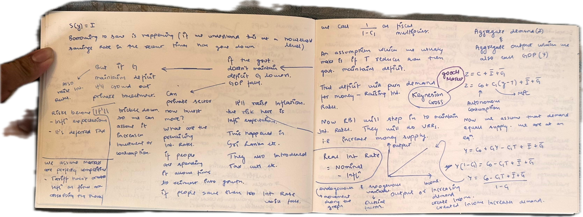
What You Can Now Do
When the next tax-cut headline lands, ask the two questions this session armed you with: what happens to G, and where does the MPC actually sit? A cut financed by lower spending is a different animal from one financed by deficit — the two scenarios carry different multipliers, and that difference is the whole argument. And when someone praises a savings drive in a slowdown, remember the paradox of thrift: individually virtuous, collectively contractionary — in the short run only.
Continue to Session 3 — Aggregate Demand & Monetary Policy, where interest rates enter the model and the RBI walks in with them.