Recap - The Keynesian Cross Model

This session begins by revisiting the fundamental aggregate demand equation that forms the foundation of Keynesian macroeconomic analysis. Understanding this model is essential for analysing how consumption, investment, and government spending interact to determine income equilibrium in the short run.

Title: Aggregate Demand Equation - Description: Screenshot showing Z = c0 + c1(y-t) + I + G

The Aggregate Demand Equation

The fundamental equation relating aggregate demand (Z) to income (Y) is:


Z = C0 + C1(Y - T) + I + G

Key Components

• Z = Aggregate Demand - total spending desired by all sectors of the economy

• C0 = Autonomous Consumption - consumption that occurs independent of income, such as from existing wealth, inheritances, or charitable contributions. This represents the baseline spending level when income is zero.

• C1 = Marginal Propensity to Consume (MPC) - the slope of the consumption function. It represents the fraction of each additional rupee of income that households consume. Range: 0 < C₁ < 1

• Y = Income (or output) - the total production of the economy

• T = Taxes - lump-sum taxes on households

• (Y - T) = Disposable Income - income remaining after tax payments, which is what households actually have available to consume or save

• I = Investment - business investment in capital. Denoted with a bar (Ī) indicating it is held constant in the initial analysis, not dependent on income

• G = Government Spending - comprises only government purchases of goods and services. Note: This does NOT include transfer payments (social security, pensions) or subsidies, as these are income transfers rather than purchases of new goods/services

Equilibrium Condition

Equilibrium in the goods market occurs when aggregate demand equals actual output:

Z = Y

Solving for equilibrium income:

Y = [C0 - C1T + I + G] / (1 - C1)

The Multiplier Effect

The denominator (1 - C¹) in the equilibrium equation gives us the reciprocal of the multiplier. An increase in autonomous spending (C⁰, I, or G) increases equilibrium income by a multiple of the initial change.

Multiplier = 1 / (1 - C¹)

Examples of Multiplier Magnitudes

• If C¹ = 50%: Multiplier = 1/(1-0.5) = 2 (a 100 rupee increase in G raises income by 200)

• If C¹ = 80%: Multiplier = 1/(1-0.8) = 5 (more consumption per rupee earned = larger multiplier)

• If C¹ = 90%: Multiplier = 1/(1-0.9) = 10 (very high savings rate leads to very large multiplier)

Real-World Application: GST Collection in India

The professor discussed a recent case with the Ministry of Finance regarding GST collection. The government expected GST revenues to grow by 11-12%, but actual growth was only 4.6%.

The Policy Question: Is it stimulative to cut taxes (T) while maintaining a balanced budget by also cutting government spending (G)?

When taxes decrease and government spending decreases equally, the net effect depends on whether the MPC of taxpayers is greater than the MPC of government spending recipients.

The Problem: There is no definitive empirical proof for which MPC is higher. The theoretical answer requires knowing the income distribution and consumption patterns of both groups.

Real Interest Rates vs Nominal Rates

A critical distinction in macroeconomics is between the nominal interest rate (what you observe) and the real interest rate (what actually matters for economic decisions). This section explains why central banks often miscalculate real rates and the consequences.

Investment as a Function of Real Interest Rate

In the more complete model, investment is no longer constant. Instead, it depends on the real interest rate R:

I = I(R)

Higher real interest rate → Lower investment

Lower real interest rate → Higher investment

The Critical Insight: Real Rates Depend on EXPECTED Inflation


Real Interest Rate = Nominal Rate - EXPECTED Inflation

This is not historical or actual inflation—it is what economic agents expect inflation to be in the future. This distinction is crucial because business investment decisions are based on expected real returns, not backward-looking inflation.

The RBI Mistake (2023-2025)

The Reserve Bank of India made a calculation error that had significant economic consequences:

What RBI Did (Incorrect):	What They Should Have Done:
Real Rate = Repo Rate - Reported Inflation 6.5% - 4.0% = 2.5%	Real Rate = Repo Rate - Expected Inflation 6.5% - 2.0-2.5% = 4.0-4.5%

Real Rate = Repo Rate - Reported Inflation

6.5% - 4.0% = 2.5%

Real Rate = Repo Rate - Expected Inflation

6.5% - 2.0-2.5% = 4.0-4.5%

Problem: RBI thought the real rate was 2.5%, when it was actually 3-4%. This is an overly restrictive real rate that no country can sustain for long periods.

Macroeconomic Consequences

• Slow Investment Growth: High real rates discourage business investment. Firms postponed capital expenditure.

• Weak Job Market: Without investment in new productive capacity, job creation slowed.

• Visible Impact on Placement: Even at ISB, placement numbers and salary offers were affected by the weak job market.

Historical Context: Normal Real Rates in India

Research on India’s history shows:

• Average Real Rate (1950s-2020s): 1.0% - 1.25%

• Neutral Real Rate: Approximately 1.75% (the rate that neither stimulates nor restricts growth)

• RBI Rate: 3-4% was deeply restrictive by historical standards

Why Real Rates Matter for Business Decisions

Businesses evaluate investment returns in real terms. Asset prices rise with inflation, so a business must earn a return above inflation to justify the investment.

Scenario A

Nominal Return: 9%

Inflation: 9%

Real Return: 0%

Verdict: No real gain

Scenario B

Nominal Return: 7%

Inflation: 4%

Real Return: 3%

Verdict: Attractive, despite lower nominal rate

Scenario B is more attractive despite the lower nominal rate because it offers a real return of 3%.

Liquidity Preference Theory - Money Demand

Money is demanded not because it generates income, but because it provides liquidity—the ability to make immediate purchases. We now develop the theory of money demand and its crucial relationship with interest rates and income.

The Money Demand Equation

M = $Y × L(i)

Money Supply = Nominal Income × Liquidity Preference Function

Components

• M = Quantity of money demanded

• $Y = Nominal income (price level × real output). Higher nominal income means more transactions, requiring more money for purchases.

• L(i) = Liquidity preference function. Shows the relationship between the interest rate and the desired ratio of money to nominal income. As interest rate rises, L(i) falls because money becomes less attractive relative to interest-bearing assets.

The Fundamental Trade-off

Holding money involves a choice between two competing forces:

Cost: Opportunity Cost

When you hold money, you forego interest income you could earn on bonds or savings accounts.

Higher interest rate → Higher opportunity cost → Hold less money

Benefit: Liquidity/Convenience

Money is immediately useful for transactions. You can buy a dosa, idli, or banana without converting assets first.

Lower interest rate → Liquidity becomes more valuable relative to foregone interest → Hold more money

Thought Experiment

Imagine an equilibrium at income = 100, interest rate = 3%, money held = 10 rupees.

Question: If income doubles to 200 but money holdings stay at 10 rupees, what must happen to interest rates?

Initial Situation:

Income = 100

Cash = 10 rupees

Cash/Income = 10/100 = 10%

After Income Doubles:

Income = 200

Cash = 10 rupees (unchanged)

Cash/Income = 10/200 = 5%

Analysis: The ratio of cash to income has fallen from 10% to 5%. This means less cash is available for transactions relative to the volume of transactions needed. People would feel inconvenience (it’s now harder to make the same purchases). This inconvenience is NOT compensated by the interest rate, which is still 3%.

Solution: Interest rates must INCREASE. The higher rate compensates for the inconvenience of holding less cash relative to income needs. Only with higher interest will people accept a lower cash-to-income ratio.

Title: Money Demand Equation - Description: Screenshot showing M = $Y × L(I) and money demand chart

Money demand equation with relationship to income and interest rates

The Same Logic Applies to Inflation

When prices double due to inflation, people need twice as much nominal cash to buy the same goods. If the central bank doesn’t supply enough money, what happens?

• If prices double but M stays constant, then M/$Y falls

• People feel less liquid (inconvenient cash situation)

• Interest rates must rise to compensate for this reduced liquidity

The Money Demand Curve

When plotted on a graph with interest rate on the vertical axis and money quantity on the horizontal axis, the money demand curve slopes downward:

• Shape: Downward sloping, like a hyperbola

• Steeper at low money quantities: Interest rates are very high. Small increases in money supply cause sharp drops in rates.

• Flatter at high money quantities: Interest rates are already low. Additional money has little effect on rates (the liquidity trap).

Shifts in the Money Demand Curve

When income increases, the entire money demand curve shifts to the right. At any given interest rate, people now want more money because they have higher income and more transactions to conduct.

Title: Income/Money Demand Relationship - Description: Screenshot showing income/money demand relationship and graph

Relationship between income and money demand with graphical representation

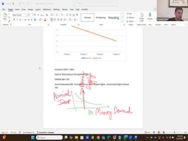
Title: Money Demand Curves - Description: Screenshot showing handwritten money demand curves with annotations

money demand curves showing shifts with income changes

Money Supply Systems - Old (IS-LM) vs New (IS-MP)

Central banks operate under different frameworks. Understanding how money is supplied to the economy and how central banks make their decisions is crucial to understanding modern monetary policy.

The Old System: IS-LM Framework

In the traditional Keynesian model (IS-LM), the central bank targets the quantity of money in the economy:

Central Bank Action:

Supply a fixed amount of money (vertical line on a graph)

Market Result:

Interest rate fluctuates based on money demand, which varies with festivals, tax seasons, and economic cycles

Problem: When demand for money spikes (e.g., during Diwali festival when people need cash for shopping), interest rates can spike sharply. When demand falls post-festival, rates plummet. This volatility can destabilize the economy.

The New System: IS-MP Framework

Modern central banks (including the RBI) target the interest rate instead:

Central Bank Action:

Set the policy interest rate (repo rate in India) at a target level (horizontal line)

Market Result:

Money supply adjusts endogenously (automatically) to match demand at the target rate

How it works: When money demand rises (festival season), the RBI supplies more money through repo operations. When demand falls, the RBI absorbs money. The interest rate stays stable at the policy rate.

Variable Rate Repo (VRR)

The RBI uses VRR auctions to supply liquidity precisely. Banks bid for rupees at the repo rate, and the RBI supplies whatever amount is demanded at that rate. This maintains interest rate stability while allowing money supply to vary.

Vulnerability: Inflation Expectations

This system has a critical vulnerability. When the RBI accommodates persistent government borrowing (supplying money to finance fiscal deficits), inflation expectations can rise if the public believes the central bank will tolerate higher inflation.

The Spiral:

1. RBI eases (lowers rates) to accommodate fiscal borrowing

2. Public sees persistent money supply growth and expects higher inflation

3. Inflation expectations rise

4. Even though RBI keeps repo rate steady, real rates INCREASE (because expected inflation is now higher)

5. This tightens monetary conditions despite RBI easing

Historical Examples of This Vulnerability

• United Kingdom (2022): After the Liz Truss government announced massive unfunded spending plans, gilt yields spiked sharply despite the Bank of England easing. Inflation expectations jumped, raising real rates.

• Venezuela: Persistent central bank accommodation of fiscal deficits led to hyperinflation and currency collapse.

• Zimbabwe: Similar pattern of monetary accommodation and loss of currency credibility.

• Pakistan: Recent experience with inflation spike following monetary accommodation of large fiscal deficits.

• Sri Lanka: Central bank accommodation of government borrowing contributed to the 2022 crisis and currency devaluation.

A central bank targeting the interest rate must maintain credibility that it will not accommodate persistent fiscal deficits indefinitely. If that credibility erodes, inflation expectations rise, real rates increase, and the accommodative policy becomes contractionary.

Takeaways

The Keynesian Aggregate Demand Model

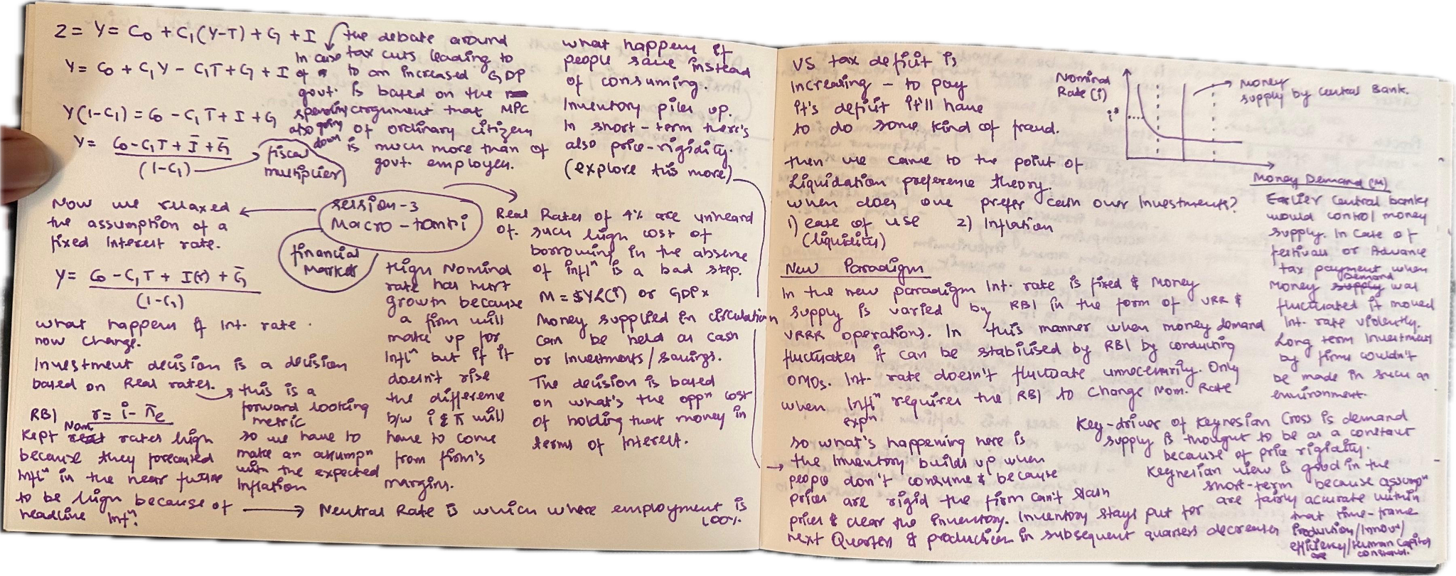
• Aggregate demand Z = C⁰ + C¹(Y-T) + I + G determines short-run equilibrium output

• The multiplier 1/(1-C¹) shows how initial spending shocks amplify into larger income changes

• Balanced budget tax cuts are not necessarily stimulative—the net effect depends on the relative MPC of different groups

Interest Rates Matter for Investment

• The real interest rate (not nominal) determines investment: Real Rate = Nominal Rate - Expected Inflation

• Businesses evaluate investment returns in real terms—they must exceed inflation to be worthwhile

• Central banks that miscalculate real rates can inadvertently create severe constraints on investment and job creation

Money Demand and Liquidity

• Money is demanded for transactions, not for income. M = $Y × L(i) captures the relationship

• Higher income raises money demand; higher interest rates lower it (due to opportunity cost)

• The money demand curve slopes downward and shifts right with income increases

Central Bank Operating Frameworks

• Old system (IS-LM): Central bank targets money supply → interest rates fluctuate

• New system (IS-MP): Central bank targets interest rate → money supply adjusts endogenously

• Vulnerability: If inflation expectations rise faster than the central bank’s credibility can contain them, real rates increase even as nominal rates stay fixed

Next Session

• Professor will combine the IS and MP curves to complete the short-term macro framework

• Analysis of how tax changes, government spending shifts, and demand shocks propagate through the economy

• Understanding the monetary policy transmission mechanism and its limitations